Basic

If we draw marbles from a bag without replacement then
- If the order matters, it is Permutation. $AB \not= BA$
- If the order does not matters, it is Combination. $ABC = ACB = CBA = ...$

\begin{align*} ^nP_{r} = \frac{n!}{(n-r)!} \\ ^nC_{r} = \frac{n!}{r!(n-r)!} \end{align*}

LOOK we divide by $n!$ because among themselves how they sit around does NOT matter! See this visualiser

When we test a probability based on information we already have in our hand is Conditional Probability.
Probability of me staying hungry tomorrow is less than I will stay hungry given I have lot of food at home!
So we shrink our sample space to the particular event.
Instead of checking how often I am hungry, we check, only those days when I had food in my fridge!

\begin{align*} P(\text{event A, GIVEN, event B}) &= \frac{P(\text{A and B})}{P(B)} \\ \implies P(A|B) & = \frac{P(A \cap B)}{P(B)} \end{align*}

I love the following visualisation for the math.

Random Variables & Distribution

There are weird random events. Welp mostly are philosophical and literal. Assume we humanly assign numbers to those random events. Then those number is our Random Variable
Random Variable are of two types
- Discrete -> Like 1 apple, 2 oranges, 3 girls. Mass function is $f(x) = P(X=x)$ while cumulative function $F(x) = P(X \lt x) = P(X=x_{1})+P(X=x_{2}) + \dots = \sum P(x) = \sum f(x)$
- Continuous -> Height, temperature, volume. Density function $P(a\leq X \leq b) = \int_{a}^bf(x)dx$ , while cumulative function is still $P(X \lt x) = F(x)$ . Note how for a single point in continuous functions, the probability is just 0.
In long term the average of independent outcomes of a random variable is its Expectation. It is an essence of the centre value of the distribution
Precisely the Probability-weighted sum of all possible values of a random variable

E[X] = \sum_{x \in X}xP(x)

The Variance is the spread of the RV from it’s centre.

\begin{align} &\text{Var}(X) = E[(X-E[X])^2] \\ \text{or, } &\text{Var}(X) = E[X^2] - (E[X])^2 \end{align}

Consequently we might need to compare two random variables and we do it with Covariance i.e. how they behave mutually.

\text{Cov}(X,Y)=E[(X-E[X])(Y-E[Y])]

Some properties of Expectation
- Linearity $E[aX+bY] = aE[X] + bE[Y]$
- Mean $E[\bar{X}] = E\left[ \frac{1}{n}\sum X_{i} \right] = \frac{1}{n}E\left[ \sum X_{i} \right]=\frac{1}{n}\sum E[X_{i}] = \frac{1}{n}\times n\times \mu = \mu$
Some properties of Variance
- Scaling & constant $\text{Var}(aX+c) = a^2\text{Var(X)}$
- Two variables $\text{Var}(X\pm Y) = \text{Var}(X)+\text{Var}(Y)\pm 2\text{Cov}(X,Y)$ i.e. if they are independent covariance is 0.
- Many variables $\text{Var}\left( \sum X_{i} \right) = \sum\text{Var}(X_{i})+2\sum_{i \lt j}\text{Cov}(X_{i},X_{j})$
- Sample mean $\text{Var}(\bar{X})=\frac{\sigma^2}{n}$
Some properties of Covariance
- $\text{Cov}(aX,bY) = ab\text{Cov}(X,Y)$
- $\text{Cov}(X,X)=\text{Var}(X)$

Discrete Distributions

Bernoulli

Ber(p) \sim f(x) = \begin{cases} p & \text{if } x = 1 \\ 1-p & \text{if } x = 0 \end{cases}

Mean is $p$ , Variance is $p(1-p)$ .
2. Binomial
Sum of n independent Bernoulli random var.

Bin(n, p) \sim f(x) = \binom{n}{x}p^r(1-p)^{n-r}

Mean is $np$ , Variance is $np(1-p)$ .
3. Geometric
It counts the number of trails that is required to observe single success. $f(x) = (1-p)^{x-1}p$ Where Mean is $1/p$ , Variance is $\frac{1-p}{p^2}$ .
4. Poisson
It counts the number of evens occurring in a fixed interval of time or space with a given average rate $\lambda$

P(\lambda) \sim f(x) = \frac{\lambda^xe^{-\lambda}}{x!}

Mean and Variance both is is $\lambda$ .

Continuous Distributions

Uniform
When all the possible intervals have equal possibility of happening.

U(a,b) \sim f(x) = \begin{cases} \frac{1}{b-a} & \text{for } x \in [a,b] \\ 0 & \text{otherwise} \end{cases}

Mean is $\frac{a+b}{2}$ , Variance is $\frac{(b-a)^2}{12}$
2. Normal
The normal (or Gaussian) is a distribution which is assumed to be additively produced by many many small effects

N(\mu,\sigma^2) \sim f(x) = \frac{1}{\sqrt{ 2\pi \sigma^2 }}e^{ - \frac{(x-\mu)^2}{2\sigma^2} }

Mean is $\mu$ , Variance is $\sigma^2$ .
3. Exponential
It is the continuous analogue of the geometric distribution.

\text{Exp}(\lambda) \sim f(x) = \begin{cases} \lambda e^{-\lambda x} & \text{if } x \geq 0 \\ 0 & \text{otherwise} \end{cases}

Mean is $1/\lambda$ , Variance is $1/\lambda^2$

The Central Limit Theorem states that the sample mean of a sufficiently large number of independent and identically distributed random variables is approximately normally distributed

Estimation

Sometimes when we obviously cant calculate a parameter, or guess its underlying distribution say a mean or something of the whole population one by one, we invent a way to Estimate them. And we create the Estimator in such a way so that it is very consistent to the actual parameter if we ever could actually measure that.
To build estimator around sampled points then using sample mean, sample variances and other sample parameters to estimate the original thing. $\bar{X} \to \mu$ etc.
In contrast to point estimation, we measure a range of possible values where the estimator will surely lie in calling it Confidence Interval
Assume we take $n$ sample points from a distribution which we don’t know yet. Then we take an confidence level of $\alpha$ then our confidence interval would be $[\theta-(1-\alpha), \theta+(1-\alpha)]$ i.e. if we measure the sample mean, the actual mean might or might not be in the interval.
Funnily if we keep taking trials and compare if it does EXIST in the interval or DOES NOT exist compared to total time. YES! PROBABILITY. We see the probability that the interval contains the actual parameter converges to $\alpha$ .
Hence, $\alpha$ is a probability measure of the existence of the true parameter in the confidence interval.
Now there can be two or more estimator for one single parameter, how do we know which one is good.
There exist computation technique called Bootstrap. We take sample and create an estimator -> Then we take a sample from that sample itself and compare over many iteration of resampling and see if the estimation is consistent.

Bayesian

Bayesian probability is a degree of belief.
“Expert says there is 60% prob someone will win in election” -> we cannot have many election to make calculation!
We cannot always think of long run frequency to test probability because it might not happen in reality.
FREQUENTIST: when a coin is flipped infinite times -> half will be heads BAYESIAN: its equally likely for next flip to be head or tails

If we flip one coin and hide the result, what is the probability THIS COIN is head? BAYESIAN: same. FREQUENTIST: no idea.
FREQUENTIST CONFIDENCE INTERVAL: We have a formula, if we repeatedly run this, 95% time its correct! BAYESIAN CREDIBLE INTERVAL: Based on everything we know, there is 95% probability that the measure is in this interval.
Bayes’ Theorem

\begin{align} P(A|B) &= \frac{P(B|A)P(A)}{P(B)} \\ \implies P(A|B)\times P(B) &= P(B|A) \times P(A) \end{align}

Intuitively what proportion when B happens then A happens as well is equal to what proportion of A happens when B happens

The plausibility of a parameter $\theta$ given the observed data $x$ is called likelihood $L(\theta|x) = P(x|\theta)$ . i.e the probability of $\theta$ has been true value and overlapped with observed $x$ in a frequentist mindset.
The core belief is “the prior belief should be updated as new data is acquired”

Regression

Least square method is one approach where we compare square of the difference of the two kind of measurements and we try to minimise the sum of the square Equation of line is $y=mx+b$ , After solving for least square we find the solution of intercept and slope with:

\begin{align} &\sum y_{i} = m\sum x_{i} + nb, \\ &\sum x_{i}y_{i} = m\sum x_{i}^2+b\sum x_{i} \end{align}

Where $n$ is sample size, $x_{i}$ & $y_{i}$ are the value of the two measurements. $m$ is slope and $b$ is intercept.

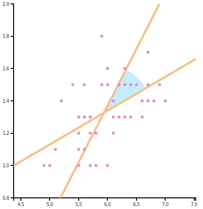
Now after finding the middle most line that separates the proportionality between the two measurement, we need a rigorous measure to compare if they increase or decrease together or what. We bring Correlation $r$ where,

r=\frac{s_{xy}}{\sqrt{ s_{xx} }\sqrt{ s_{yy} }}

and $s_{xy}, s_{xx}, s_{yy}$ are defined as:

\begin{align} s_{xy} &= \sum(x_{i}-\bar{x})(y_{i}-\bar{y}) \\ s_{xx} &= \sum(x_{i}-\bar{x})^2 \\ s_{yy} &= \sum(y_{i}-\bar{y})^2 \end{align}

note, r lies between -1 and 1, and 0 means no correlation. It is actually intuitively, cosine of the angle between when we take the regression lines made by least square $Y_{xy}$ i.e the line of $x$ wrt to $y$ , and $Y_{yx}$ i.e the line of $y$ wrt to $x$ .

diag from seeing theory

Comparison

Cohen’s d is standardised way to test how big the difference is.

\begin{align} d &= \frac{\mu_{1}-\mu_{2}}{\text{pooled }SD} \\ \text{pooled SD} &= \sqrt{ \frac{(n_{1}-1)\times SD_{1}^2 + (n_{2}-1)\times SD_{2}^2}{n_{1}+n_{2}-2} } \end{align}

Hypothesis Testing

We create a hypothesis to fight two independent concept. Data gives evidence hypothesis is wrong -> we reject the hypothesis Data similar but not same -> fail to reject

Hypothesis could have been anything based on different sample. So we take the trivial case of assuming, there is no difference between the two concept. This is called the Null Hypothesis $H_{0}$ . We also take an Alternative Hypothesis $H_{1}$ where we just assume there exists a difference and we fight those two hypothesis together.
We put our need as $H_{1}$ and test with contradiction method assuming $H_{0}$ is true then, $E(\hat{\theta})=0 \to$ because the two measurement have no difference $V(\hat{\theta}) = V(p_{1}-p_{2}) = V(p_{1})+V(p_{0}) = \frac{p(1-p)}{n_{1}}+\frac{p(1-p)}{n_{0}} = p(1-p)\left( \frac{1}{n_{1}} + \frac{1}{n_{0}} \right) \to$ because the outcome are not supposed to have any differences! So consequently since the individual tests are just bernoulli intuitively we can say using the CLT,

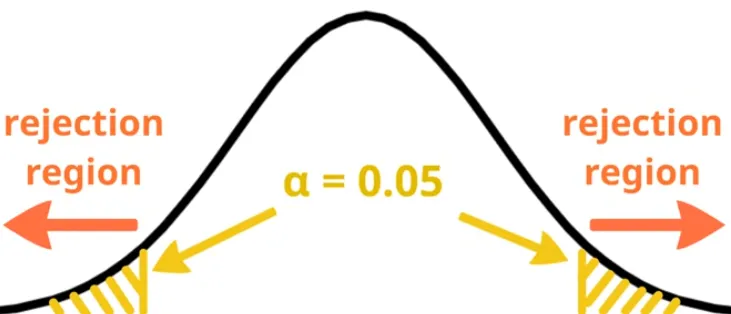
\hat{\theta} \sim N\left( 0,p(1-p)\left( \frac{1}{n_{1}}+\frac{1}{n_{0}} \right) \right)

But since normal distribution is continuous $(-\infty, +\infty)$ , we must define an interval within which we accept the null hypothesis; otherwise, even very small differences could lead us to reject it. The size of probability for which we must reject the $H_{0}$ is called the level of significance $\alpha$
T-Statistics
Consider the test statistic

T = \frac{\hat{\theta}}{SE(\hat{\theta})}=\frac{\hat{\theta}}{\sqrt{ p(1-p)\left( \frac{1}{n_{1}}+\frac{1}{n_{0}} \right) }}

then we see, $E(T) = 0, \text{Var}(T)=1$ , i.e $T\sim N(0,1)$ The critical value i.e. the value at the edge of the level of significance is mostly given and with our sample we only calculate $t$ to test if the $H_{0}$ can be rejected or not.

Nothing can be ever proven it can only be inferred.
If $H_{0}$ is true, then if we do the same experiment repeatedly, the test statistics will vary. The probability under that null distribution, of getting a test statistics at least as far from the null value which we observed.

\begin{align} p &= P(|T|\geq |t_{\text{obs}}||H_{0}) \\ \text{or, } p&= 2P(Z\geq|t_{\text{obs}}|) \end{align}

We always test against both are same, now we reverse ask, for what kind of differences there wouldn’t be much separation? So, we have $Z=\frac{\hat{\theta}-\theta}{SE} \sim N(0,1)$ , And we can also compute for 95% confidence we need, $c$ such that $P(-c \lt Z \lt c) = 0.95$ where our assumed $\alpha$ is 0.05%, by using the normal distribution function we can calculate $c=1.96$ , so if we use these information,

\begin{align} P(-1.96 \lt Z \lt 1.96) = 0.95 \\ \text{or, } P(-1.96 \lt \frac{\hat{\theta}-\theta}{SE} \lt 1.96) = 0.95 \\ \text{or, } P(\hat{\theta}-1.96SE \lt \theta \lt \hat{\theta}+1.96SE) = 0.95 \\ \\ \end{align}

e.i. the confidence interval of 95% is $\hat{\theta}\pm1.96SE$ .

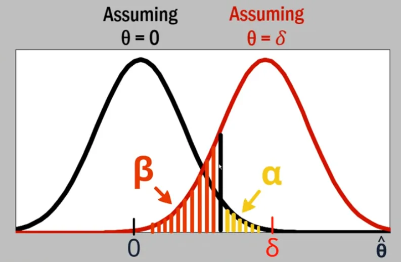
Power is the probability of rejecting a FALSE $H_{0}$ i.e. the ability of a model to detect a specified difference, $\delta$

	Accept $H_{0}$	Reject $H_{0}$
$H_{0}$ is true	True -ve 1- $\alpha$	False +ve $\alpha$ Type I error
$H_{0}$ is false	False -ve $\beta$ Type II error	True +ve $1-\beta$ Power

zed stat

Notes: Statistics Refresher for Machine Learning